Entry 1: fs2, gRPC, Triton Inference Server

Posted Nov 4, 2023 Updated Nov 27, 2023

By Matt Langsenkamp 31 min read

Overview

This is the second post in a series about inference of machine learning models using scala. The first post can be found here. This post will detail how to use a functional streaming library (fs2) to perform machine learning model inference using the Triton Inference Server and gRPC. The post will be broken up into a few different parts. First we will set up our scala, python and docker dependencies. Then we will get Triton up and running using Docker. Finally we will set up fs2 to read from a text file containing image paths. We will use opencv to format our images into the representation Triton expects. Finally we will load images and send them to Triton in batches, displaying the result to the console.

The github repo for these tutorials can be found here

Setup

It is expected that you have the following tools installed:

scala build tool sbt
python build tool poetry
Cuda toolkit and Nvidia Docker. More detailed installation tips can be found in the github readme

Scala and File Directory

First create a new project using the scala 3 giter template/sbt and move to the newly created directory.

  
sbt new scala/scala3.g8
#   name [Scala 3 Project Template]: scalamachinelearningdeployment
#   Template applied in ./scalamachinelearningdeployment
cd scalamachinelearningdeployment

Next we will add the fs2 gRPC plugin. Add the following to project/plugins.sbt. This is what will turn our .proto files into code we can use to talk with Triton. We will talk more about .proto files and gRPC later.

  
addSbtPlugin("org.typelevel" % "sbt-fs2-grpc" % "2.7.4")

We then need to create a module to store our .proto files in, and to run code generation from.

mkdir -p protobuf/src/main/protobuf/

Create a file called downloadprotos.sh and add the following content. These are the proto files provided by the Triton Inference Server. They allow for us to communicate with Triton in any language that can generate code from .proto files.

  
for PROTO in 'grpc_service' 'health' 'model_config'
do
    wget -O ./protobuf/src/main/protobuf/$PROTO.proto https://raw.githubusercontent.com/triton-inference-server/common/main/protobuf/$PROTO.proto
done

Then run the script to download the files.

chmod +x downloadprotos.sh
./downloadprotos.sh

Finally we need to configure our build.sbt. There are a couple key steps to make note of:

Create variables to manage our dependencies
Create a module for the protobuf subdirectory, explicitly stating we depend on the gRPC plugin
Add our dependencies to our root module and make the root module depend to the protobuf module

  
// 1 create dependency variables
val scala3Version = "3.3.1"
val fs2Version    = "3.9.3"
val openCVVersion = "1.5.9"
val circeVersion  = "0.14.6"
val osLibVersion  = "0.9.2"

// 2 create protobuf module
lazy val protobuf =
  project
    .in(file("protobuf"))
    .settings(
      name         := "protobuf",
      scalaVersion := scala3Version
    )
    .enablePlugins(Fs2Grpc) // explicitly depend on gRPC plugin

lazy val root = project
  .in(file("."))
  .settings(
    name         := "scalamachinelearningdeployment",
    version      := "0.0.1",
    scalaVersion := scala3Version,
    // 3 add dependencies
    libraryDependencies ++= Seq(
      "io.grpc"        % "grpc-netty-shaded" % scalapb.compiler.Version.grpcJavaVersion,
      "co.fs2"        %% "fs2-core"          % fs2Version,
      "co.fs2"        %% "fs2-io"            % fs2Version,
      "org.bytedeco"   % "javacv-platform"   % openCVVersion,
      "io.circe"      %% "circe-core"        % circeVersion,
      "io.circe"      %% "circe-generic"     % circeVersion,
      "io.circe"      %% "circe-parser"      % circeVersion,
      "com.lihaoyi"   %% "os-lib"            % osLibVersion,
      "org.scalameta" %% "munit"             % "0.7.29" % Test
    ),
    fork := true
  )
  .dependsOn(protobuf) // explicitly depend on protobuf module

Compile your code with sbt compile to make sure everything went smoothly

Python and ONNX Models

I use the poetry package manager to manage my python dependencies but you can modify these instructions if you want to use something else.

  
poetry init
# Package name [scalamachinelearningdeployment]:  
# Version [0.1.0]:  0.0.1
# Description []:  
# Author [Nyour name> <your email>, n to skip]:  n
# License []:  
# Compatible Python versions [^3.10]:  

# Would you like to define your main dependencies interactively? (yes/no) [yes] no
# Would you like to define your development dependencies interactively? (yes/no) [yes] no

A .pyproject.toml file will be created after all the prompts have been completed. Add the following lines to the dependencies section.

  
[tool.poetry.dependencies]
python = ">=3.10,<3.13"
onnxruntime-gpu = "^1.16.0"
torch = "^2.0.0"
ultralytics = "^8.0.190"
onnxruntime = "^1.16.0"
onnx = "^1.14.1"
pillow = "^10.1.0"

Then run poetry install to download our dependencies. We can now start writing our script to download and pre-process our models. Our script will do the following:

Download a pre-trained yolov8 model from ultralytics.
Convert the model to ONNX format, saving copies in batch sizes of 1 and 16
Inspect the input and outputs of our ONNX model
Save output mapping in the model to JSON format so that we can use it from scala

  
mkdir -p src/main/python
touch src/main/python/preprocess_model.py

  
from ultralytics import YOLO
from onnx import load
import os
import json


if __name__ == "__main__":
    # 1 This will automatically download the model from the ultralytics repo
    orig_model = YOLO("yolov8n-cls.pt")

    # 2 export model to onnx format in batch sizes 1 and 16
    orig_model.export(format="onnx")
    os.rename("yolov8n-cls.onnx", "yolov8n-cls-1.onnx")
    orig_model.export(format="onnx", batch=16)
    os.rename("yolov8n-cls.onnx", "yolov8n-cls-16.onnx")

    # 3 inspect inputs and outputs
    model = load("yolov8n-cls-1.onnx")

    print(
        "\n\n --- inspecting model inputs and outputs of model with batch size 1 --- "
    )
    print(" --- inputs ---")
    i = model.graph.input[0]
    print(i)
    print(" --- outputs ---")
    o = model.graph.output[0]
    print(o)
    print(" ------------------------------------------- \n\n")

    model = load("yolov8n-cls-16.onnx")

    print(
        "\n\n --- inspecting model inputs and outputs of model with batch size 16 --- "
    )
    print(" --- inputs ---")
    i = model.graph.input[0]
    print(i)
    print(" --- outputs ---")
    o = model.graph.output[0]
    print(o)
    print(" ------------------------------------------- \n\n")

    # 4 save the label lookup table
    lookup_dict = eval(model.metadata_props[-1].value)
    with open("labels.json", "w") as outfile:
        json.dump(lookup_dict, outfile)

poetry shell
python src/main/python/preprocess_model.py

After running the script we will see the following output for the model we created with a batch size of 1. Each output has a name field and a type field. The type field describes the shape of the input or output tensor. We can see that this model expects and input shape of [1, 3, 224, 224]. In other words the input is 1 image with three channels (RGB) with a height and width of 224. The output is a tensor of shape [1, 1000]. This corresponds to a single vector of 1000 different indices, each of which corresponds to a label. The values of these indices will range from 0 to 1, with values closer to 1 indicating that the model believes the image represents the label corresponding to this index. This will make more sense when we examine the label map.

--- inputs ---
name: "images"
type {
  tensor_type {
    elem_type: 1
    shape {
      dim {
        dim_value: 1
      }
      dim {
        dim_value: 3
      }
      dim {
        dim_value: 224
      }
      dim {
        dim_value: 224
      }
    }
  }
}

 --- outputs ---
name: "output0"
type {
  tensor_type {
    elem_type: 1
    shape {
      dim {
        dim_value: 1
      }
      dim {
        dim_value: 1000
      }
    }
  }
}

When observing the model with a batch size of 16 we can see that all is the same except now that instead of 1 image as input and 1 tensor of 1000 as output, we have 16 input images and 16 tensors of 1000 as output. Batches of 1 and 16 where chosen somewhat arbitrarily, simply to highlight that this functionality is possible. The optimal batch size for your deployment will have to be found by running benchmarks.

 --- inputs ---
name: "images"
type {
  tensor_type {
    elem_type: 1
    shape {
      dim {
        dim_value: 16
      }
      dim {
        dim_value: 3
      }
      dim {
        dim_value: 224
      }
      dim {
        dim_value: 224
      }
    }
  }
}

 --- outputs ---
name: "output0"
type {
  tensor_type {
    elem_type: 1
    shape {
      dim {
        dim_value: 16
      }
      dim {
        dim_value: 1000
      }
    }
  }
}

The last piece of our pre-process script we need to discuss is the lookup table extracted from the ONNX metadata. ONNX allows metadata to be stored with the model to make it as portable as possible. In this case that means providing a mapping from each of the 1000 indices in the output tensor to their label. Below is an abbreviated version of said mapping.

  
{
  "0": "tench", 
  "1": "goldfish", 
  "2": "great_white_shark", 
  "3": "tiger_shark",
  ...
  "997": "bolete", 
  "998": "ear", 
  "999": "toilet_tissue"
}

If the returned 1000 index tensor related to an input image had a value of 0.9 at index 3 and values <0.1 for every other index, we would take that to mean that the predicted value of said image, is a tiger shark.

Triton container setup

Triton Inference Server is a versatile tool for serving trained machine learning models. Its feature set includes but is not limited to:

multiple flavors of dynamic batching
multiple backend implementations
gRPC and HTTP endpoints
serving multiple models at a time, using different backends
swapping out models without restarting
pipelines in order to limit RPC calls
tools for performing parameter pruning to discover optimal deployment strategy

We will not cover all of these topics here as that would turn this into a very long post. Instead we will focus on a simple deployment which makes use of two models, one which expects a batch-size of 1 and one which can except a batch size of 16. Both of these models will target the TensorRT backend, and will be loaded at the same time and will be wrapped in a Docker container for ease of deployment. If you want to learn more about Triton the concepts tutorial and architecture overview documentation pages are good places to start.

The Triton server is a configuration driven tool. It expects to have access to a directory that is formatted a certain way, with specific files in specific places with in said directory. As an example see the diagram below

models
├──yolov8_1
│  ├──config.pbtxt
│  ├──1
│  │  ├──model.onnx
├──yolov8_16
│  ├──config.pbtxt
│  ├──1
│  │  ├──model.onnx

There is a top level directory models which contains the subdirectories for the two models we will deploy. yolov8_1 is the model which contains a batch size of 1. within this directory is a config.pbtxt file which contains information on how Triton will deploy this model as well as a directory named 1 containing the model itself. The 1 directory represents the first version of this model. As development and refinement of the model progresses more directories such as 2, 3, etc. can be added. The models that are actually deployed can be determined by a field set in config.pbtxt. We will only have one version to deploy so we can omit that field

Below is the config.pbtxt for the model with a batch size of 16. The config for the model with a batch size of 1 is the same but with the batch sizes set to 1. If you have followed the discussion about ONNX models thus far the input and output fields should make perfect sense. The max_batch_size field is set to 0, which just means that it will defer to the leading dimension of the model itself as the batch size. The backend field is set to tensorrt which indicates that the model will use the TensorRT engine. The last part of the config file that requires explanation is the model_warmup field. Often parts of neural networks are initialized lazily, meaning that the whole graph is not fully loaded until it receives some initial data. This means the first request will experience significantly higher latency than all subsequent requests. The model warmup simply sends some garbage data to the model to trigger any lazy loading which might happen.

name: "yolov8_16"
backend: "tensorrt"
max_batch_size : 0
input [
  {
    name: "images"
    data_type: TYPE_FP32
    dims: [ 16, 3, 224, 224 ]
  }
]
output [
  {
    name: "output0"
    data_type: TYPE_FP32
    dims: [ 16, 1000 ]
  }
]

model_warmup {
   name: "text_recognition"
   batch_size: 0
   inputs: {
       key: "images"
       value: {
           data_type: TYPE_FP32
           dims: 16
           dims: 3
           dims: 224
           dims: 224
           zero_data: true
       }
   }
}

Triton has the ability to automatically convert ONNX models to TensorRT .plan model types, however this process causes a delay in our service going live. This delay is only a couple seconds, but in scenarios where services need to dynamically be scaled up and down, a couple seconds is likely unacceptable. To mitigate this we will use the trtexec util provided by the TensorRT containers to convert the models beforehand.

Run the following command to run bash within the TensorRT container. Note that we are making use of a docker volume so we automatically have access to all the files and folders in our project.

  
docker run --gpus all -it -v $(pwd)/:/workspace --rm nvcr.io/nvidia/tensorrt:23.10-py3 bash

Once inside the newly started session run

  
trtexec --onnx=yolov8n-cls-1.onnx --saveEngine=yolov8n-cls-1.plan --explicitBatch
trtexec --onnx=yolov8n-cls-16.onnx --saveEngine=yolov8n-cls-16.plan --explicitBatch

Now that we our fully prepared TensorRT .plan models we can create our Triton dockerfile. We will use the Triton dockerfile provided by Nvidia for our base file, and simply format the model the model repository directory as we discussed earlier and point the tritonserver command at said repository. Create a file called .Dockerfile and add the following contents.

  
FROM nvcr.io/nvidia/tritonserver:23.10-py3

RUN mkdir -p models/yolov8_1/1/
COPY config_1.pbtxt models/yolov8_1/config.pbtxt
COPY yolov8n-cls-1.plan models/yolov8_1/1/model.plan

RUN mkdir -p models/yolov8_16/1/
COPY config_16.pbtxt models/yolov8_16/config.pbtxt
COPY yolov8n-cls-16.plan models/yolov8_16/1/model.plan

CMD [ "tritonserver",  "--model-repository=/opt/tritonserver/models" ]

Next build and run the docker image with the following commands

  
docker buildx build -t tritondeployment .
docker run --gpus all -p 8000:8000 -p 8001:8001 -p 8002:8002 --rm tritondeployment

Building fs2 Streams

Our stream will consist of three aspects:

Loading the images into a stream
preprocessing the images
sending the images to Triton via gRPC

Image Preprocessing

We will start by talking a bit about how opencv stores images and defining our image preprocessing function, as having this function handy will make creating the stream easier. Opencv by default reads color images as BGR (Blue, Green, Red), instead of in RGB format. Opencv stores the pixel values associated with each image as a single flat buffer for performance reasons. The first 3 elements of this buffer will correspond to the blue, green and red channels of the first pixel, respectively. The next three pixels will correspond to the second pixel, with the next three corresponding to the third pixel and so on. Our gRPC call however expects a different layout of the pixel values. Instead it expects all of the red pixel then all of the green pixel value and finally all of the blue pixel values. Luckily opencv provides utilities for resizing our image and converting it to RGB format.

As an example consider the three images below. The first is how we conceptually model a 3x3 RGB image. Each pixel has a red, blue and green channel and the pixels are divided into rows and columns. Each channel within a pixel contains an integer value from [0-255]. The second image is how opencv stores the image. It is the same values as what is described in the first image just flattened out. Then we have the last image which is what Triton expects. It is all the values from the red channel, then the blue channel and finally the green channel all normalized to float values [0-1]. 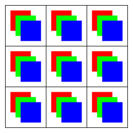The conceptual model we use when thinking about images The internal format used by opencv Mat image container, after converting to RGB format The format onnx expects via the gRPC call, which it will reshape at the server

Below is the code that converts our opencv Mat into a scala Vector with the data formatted as shown in the third image. Create a file called src/main/scala/OpenCVUtils.scala and put the following contents in there.

  
import org.bytedeco.opencv.opencv_core.Mat
import org.bytedeco.opencv.opencv_core.Size
import org.opencv.core.CvType
import org.bytedeco.opencv.global.opencv_imgcodecs._
import org.bytedeco.opencv.global.opencv_imgproc.{cvtColor, resize, COLOR_BGR2RGB}
import org.bytedeco.javacpp.indexer.{UByteRawIndexer, FloatRawIndexer}

object OpenCVUtils {

  def mat2Seq(loadedMat: Mat): Vector[Float] =
    // resize matrix
    val intMat = new Mat()
    resize(loadedMat, intMat, new Size(224, 224))
    // convert datatype to float
    val floatMat = new Mat()
    intMat.convertTo(floatMat, CvType.CV_32FC3)
    // convert BGR to RGB
    val mat = new Mat()
    cvtColor(floatMat, mat, COLOR_BGR2RGB)

    // order data based on channels
    val rows             = mat.rows
    val cols             = mat.cols
    val channels         = mat.channels()
    val pixelsPerChannel = rows * cols

    val resultArray = new Array[Float](rows * cols * channels)
    val indexer     = mat.createIndexer[FloatRawIndexer]()
    val data        = new Array[Float](channels)
    for (r <- 0 until rows)
      for (c <- 0 until cols)
        indexer.get(r, c, data)
        val channelPixel = rows * c + r
        val rPixelIndex  = channelPixel
        val gPixelIndex  = channelPixel + pixelsPerChannel
        val bPixelIndex  = channelPixel + 2 * pixelsPerChannel
        // normalize data
        resultArray(rPixelIndex) = data(0) / 255
        resultArray(gPixelIndex) = data(1) / 255
        resultArray(bPixelIndex) = data(2) / 255
    resultArray.toVector
}

Stream Building

We need to download the data we will be processing in our stream. Download the images and extract them below with the following commands

  
wget https://github.com/MattLangsenkamp/scala-machine-learning-deployment/raw/main/data.tar.xz
tar -xf data.tar.xz
mv ./data/* ./

The first part of building our stream is understanding our data source. When we view the contents of images.txt we can see that each line is a tuple of a path to an image, and its ground truth label. These images and their labels where selected from the image-net dataset.

images/grocery_store.jpeg grocery_store
images/Chihuahua.jpeg Chihuahua
images/goldfish.jpeg goldfish
images/ambulance.jpeg ambulance
images/scorpion.jpeg scorpion
images/snowmobile.jpeg snowmobile
images/pineapple.jpeg pineapple
images/syringe.jpeg syringe
images/screwdriver.jpeg screwdriver
images/radio.jpeg radio

Before we can start writing our stream we need to create a file and add some dependencies. Create src/main/scala/Main.scala and add the following code

  
import cats.implicits.*
import cats.effect.*
import cats.effect.IO.*
import cats.effect.implicits.*
import io.grpc.netty.shaded.io.grpc.netty.NettyChannelBuilder
import io.grpc.*
import fs2.grpc.syntax.all.*
import fs2.{Stream, text}
import fs2.io.file.{Files, Path}
import inference.grpc_service.{
  GRPCInferenceServiceFs2Grpc,
  ModelInferRequest,
  ModelInferResponse,
  InferTensorContents
}
import inference.grpc_service.ModelInferRequest.InferInputTensor
import os.{GlobSyntax, /, read, pwd}
import org.bytedeco.opencv.global.opencv_imgcodecs._
import org.bytedeco.opencv.global.opencv_imgproc.resize
import org.bytedeco.opencv.opencv_core.{Mat, Size}
import org.opencv.core.CvType
import OpenCVUtils.mat2Seq

import java.nio.ByteOrder

object GrpcClient extends IOApp.Simple:
  // all following code snippets go here!

Recall that we now have our image pre-process function, so we now have the ability to do the following

Read images.txt line by line
convert each line into a tuple of path and label
Read the image at each path and pre-process it, keeping its label attached to it.

The code below does just this. Note that the image reading and pre-processing step is wrapped in a blocking IO as reading the image and performing the computations is a blocking IO effect.

  
def getImageStream(batchSize: Int) = Files[IO]
  .readAll(Path((pwd / "images.txt").toString))
  .through(text.utf8.decode)
  .through(text.lines)
  .map(l =>
    val pathAndLabel = l.split(' ')
    (pathAndLabel(0), pathAndLabel(1))
  )
  .evalMap((path, label) =>
    IO.blocking {
      val img = imread((pwd / os.RelPath[String](path)).toString)
      (mat2Seq(img), label)
    }
  )

Remember earlier that we created two versions of our model, one with batch size of 1 and another of 16. We need to add to our stream so that it can create arbitrarily sized batches of inference requests. To do so add the following calls to the fs2 stream we just created:

  
  .chunkN(batchSize, allowFewer = true)
  .map(chunk =>
    chunk.foldLeft(Vector.empty[Float], Vector.empty[String]) { 
      case ((lf, ls), (lf2, s)) =>
        (lf ++ lf2, ls :+ s)
    }
  )

This will take our stream of (Vector[Float], String) and convert it into a stream of (Vector[Float], Vector[String]) where the vector of floats represents all of the float vectors representing images in a batch concatenated into one vector, in order. The vector of strings is the labels of these images in the same order. Triton server will be able to decode this one big float into the correct shape as the model we provide it will have a shape of [batchsize, 3, 224, 224]

Our data is now in the format that gRPC expects… well kind of. We first need to create a function that will wrap all of vectors in objects that gRPC can make sense of. To do so add the following function:

  
def makeModelInferRequest(floatVec: Vector[Float], batchSize: Int): ModelInferRequest =
  val ic = InferTensorContents(fp32Contents = floatVec)
  val it = InferInputTensor("images", "FP32", Seq(batchSize, 3, 224, 224), contents = Some(ic))
  ModelInferRequest(s"yolov8_$batchSize", "1", inputs = Seq(it))

Then we use this function to turn our stream of (Vector[Float], Vector[String]) to a stream of (ModelInferRequest, Vector[String]) by adding the following call

  
  .map((seq, labels) => (makeModelInferRequest(seq, batchSize), labels))

This code puts our image vector in an InferTensorContents case class, which is then put in the InferInputTensor case class. Other inputs to InferInputTensor class are the input name, the datatype and the shape of the data. Note that this input name is the same as what was displayed when we inspected our ONNX model earlier. This is not by accident, as this is how Triton will know what to do with this Tensor. Finally we add the tensor as input to a ModelInferRequests case class along with the model we are targeting along with the model version. Again note that as along as we pass a batch size of 1 or 16 s"yolov8_$batchSize" will resolve to one of the models we set up with Triton.

This is now a good time to talk about gRPC and code generation. You may be looking at the previous code snippet and thinking “where did those case classes come from?”. We did not have any dependencies in our build.sbt about specifically about Triton so how do we get these case classes? In fact they where build by the sbt-fs2-grpc plugin and the .proto files we downloaded at the beginning of this post.

Protocol buffers are a format created by Google for efficient cross-platform data serialization. It knows how to serialize this data based on the definition of message structures that are defined in .proto files. We will not go over the exact syntax of protocol buffer messages as the official documentation does a good enough job of that. Instead we will look at the .proto files we downloaded early. The snippet below shows the message that was used to create our InferTensorContents, InferInputTensor and ModelInferRequest` case classes we used earlier.

  
message InferTensorContents
{
  repeated bool bool_contents = 1;

  repeated int32 int_contents = 2;

  repeated int64 int64_contents = 3;

  repeated uint32 uint_contents = 4;

  repeated uint64 uint64_contents = 5;

  repeated float fp32_contents = 6;

  repeated double fp64_contents = 7;

  repeated bytes bytes_contents = 8;
}

message ModelInferRequest
{
  message InferInputTensor
  {
    string name = 1;

    string datatype = 2;

    repeated int64 shape = 3;

    map<string, InferParameter> parameters = 4;

    InferTensorContents contents = 5;
  }

  message InferRequestedOutputTensor
  {
    string name = 1;

    map<string, InferParameter> parameters = 2;
  }

  string model_name = 1;

  string model_version = 2;

  string id = 3;

  map<string, InferParameter> parameters = 4;

  repeated InferInputTensor inputs = 5;

  repeated InferRequestedOutputTensor outputs = 6;

  repeated bytes raw_input_contents = 7;
}

If we look at each of the message definitions in protobuf/src/main/protobuf/grpc_service we see that the defined fields match exactly with a field in the case class. The generated case classes reside in protobuf/target/scala-3.3.1/src_managed/main/fs2-grpc/inference/grpc_service/GRPCInferenceServiceFs2Grpc.scala and are not just case classes but also have all of the functionality implemented needed to serialize the case classes into protocol buffers.

gRPC builds off of Protocol Buffers but adds the concept of a service and an rpc, which stands for remote procedure call. A service is similar to what scala would define as an object and an rpc can be thought of as a function defined for that object. Again we will not cover the syntax in detail as that is handled well by the documentation. This lets us define the services in .proto and our code generation tool will build the clients for free and provide us with signatures of services to implement. Below is the a shortened version of the service we will use to talk to Triton defined in protobuf/src/main/protobuf/grpc_service.

  
service GRPCInferenceService
{

  // other rpc calls removed for brevity

  rpc ModelInfer(ModelInferRequest) returns (ModelInferResponse) {}

  // other rpc calls removed for brevity

}

Its signature is pretty straight forward. It simply defines an rpc, which takes a ModelInferRequest message and returns a ModelInferResponse message. When code generation is run this translate to a Scala class which has a method that takes a ModelInferRequest case class and returns a ModelInferResponse case class. Lucky for us we have already created a stream of ModelInferRequest. Now all we need to do is get a client up and running. Using the java based gRPC client and the extension methods provided by fs2.grpc we are able to do just that.

  
val grpcStub: Resource[IO, GRPCInferenceServiceFs2Grpc[IO, Metadata]] =
  NettyChannelBuilder
    .forAddress("127.0.0.1", 8001)
    .usePlaintext()
    .resource[IO]
    .flatMap(GRPCInferenceServiceFs2Grpc.stubResource[IO])

We are now ready to define our run method which will be the entrypoint to the cats-effect runtime.

  
def run =
  val batchSize = 1 // 1 or 16
  grpcStub.use(s =>
    getImageStream(batchSize)
      .evalMap((mir, labels) => s.modelInfer(mir, new Metadata()).map((_, labels)))
      .printlns
      .compile
      .drain
  )

Assuming the instance of Triton Inference Server we started earlier is still up and running all we should need to do is run sbt run and we should see the following output below.

  
[info] (ModelInferResponse(yolov8_1,1,,Map(),Vector(InferOutputTensor(output0,FP32,Vector(1, 1000),Map(),None,UnknownFieldSet(Map()))),Vector(<ByteString@171eeb97 size=4000 contents="\273\"\\2\242\315\0275\225\315P6\324\367\0263=\342\2345\031\334\3525\324\316#3\243\351\0337O\02275\374b\2073\334\377$5\352:\225...">),UnknownFieldSet(Map())),Vector(grocery_store))
[info] (ModelInferResponse(yolov8_1,1,,Map(),Vector(InferOutputTensor(output0,FP32,Vector(1, 1000),Map(),None,UnknownFieldSet(Map()))),Vector(<ByteString@5097a3ad size=4000 contents="\275R\3733\276H\2067\247[\3323\f\315\2602\032\223\2604\ay\2746Z\371\2255\222\345\t5\314U\a7\302\315r39r\\7\275C\017...">),UnknownFieldSet(Map())),Vector(Chihuahua))
[info] (ModelInferResponse(yolov8_1,1,,Map(),Vector(InferOutputTensor(output0,FP32,Vector(1, 1000),Map(),None,UnknownFieldSet(Map()))),Vector(<ByteString@5e5047cf size=4000 contents="\255Z\2377\210_\367>o\273Z8c\311\003:\023\360\2519^\255f;\252\277\023<\246\256\2227\026\003!7:ff3t\340\2058\301$d...">),UnknownFieldSet(Map())),Vector(goldfish))
[info] (ModelInferResponse(yolov8_1,1,,Map(),Vector(InferOutputTensor(output0,FP32,Vector(1, 1000),Map(),None,UnknownFieldSet(Map()))),Vector(<ByteString@4af133e8 size=4000 contents="`.)4\256\273\0166\025\360\b6\005d83a\374\0246H_\2024\211\321;3t\317\3474!1\0235\242\244\2235K\254\20041\232\267...">),UnknownFieldSet(Map())),Vector(ambulance))
[info] (ModelInferResponse(yolov8_1,1,,Map(),Vector(InferOutputTensor(output0,FP32,Vector(1, 1000),Map(),None,UnknownFieldSet(Map()))),Vector(<ByteString@63edbccb size=4000 contents="]\215\2776 \351\2725\"N\3672\201\016D4=W\2435=\351$7\0019\0306\250\005\2637L\266m6\334\322\3173\2459U8\n\233\302...">),UnknownFieldSet(Map())),Vector(scorpion))
[info] (ModelInferResponse(yolov8_1,1,,Map(),Vector(InferOutputTensor(output0,FP32,Vector(1, 1000),Map(),None,UnknownFieldSet(Map()))),Vector(<ByteString@489b8a3b size=4000 contents="\345\332\v9WH\0027CN38\206\320\3037\224\a\"8\314\323Y5\2760\2376X\325,8\221\256\0317\372\337*3Up#5\321\356\246...">),UnknownFieldSet(Map())),Vector(snowmobile))
[info] (ModelInferResponse(yolov8_1,1,,Map(),Vector(InferOutputTensor(output0,FP32,Vector(1, 1000),Map(),None,UnknownFieldSet(Map()))),Vector(<ByteString@6947a7d2 size=4000 contents="\366\n\3544j\020V7\202\361c6e\337o2?\276\2744\031(\2064p\321\2035\336\310^9\274\375\3438\376\354X6\205\270\0328\003\031\037...">),UnknownFieldSet(Map())),Vector(pineapple))
[info] (ModelInferResponse(yolov8_1,1,,Map(),Vector(InferOutputTensor(output0,FP32,Vector(1, 1000),Map(),None,UnknownFieldSet(Map()))),Vector(<ByteString@22413634 size=4000 contents="\202\226\3724\333\363\2404\f\207\2405\234\r\3363\374\356p6S\223\2624@2\3653\027\27145\376f64!z25\300I\3226p\242c...">),UnknownFieldSet(Map())),Vector(syringe))
[info] (ModelInferResponse(yolov8_1,1,,Map(),Vector(InferOutputTensor(output0,FP32,Vector(1, 1000),Map(),None,UnknownFieldSet(Map()))),Vector(<ByteString@68630b68 size=4000 contents="\216:73\005^?4\353\235\f4J,h1\3217\0205D\216\0043\263:\2571\307^\3702G\311\2741\341\243\0363\220\362\2153\273k\334...">),UnknownFieldSet(Map())),Vector(screwdriver))
[info] (ModelInferResponse(yolov8_1,1,,Map(),Vector(InferOutputTensor(output0,FP32,Vector(1, 1000),Map(),None,UnknownFieldSet(Map()))),Vector(<ByteString@47d665d7 size=4000 contents="\313\227\2551\317\a\3402y\272\3362\232\016B2(\261#1\305\354>3\212;#2RZ\2413\006\212^2\267Pf2uy\2412\r\330\252...">),UnknownFieldSet(Map())),Vector(radio))

This is promising as we are seeing that we have a ModelInferResponse for each request, with a vector of InferOutputTensor. However when we examine the contents field of this InferOutputTensor we see that the data returned is just a raw byte string, which doesn’t the humans on the other side of this request. We now need to create a method that can decode this response into something that makes sense to humans.

To do this we will need to do the following:

Decode the bytes string into a single array of floats
Split up the single array of floats into segments of 1000, each representing a single image
Lookup the label predicted labels using the LabelMap we created earlier.

  
def decodeModelInferResponse(
    response: ModelInferResponse,
    batchSize: Int,
    topK: Int,
    labelMap: LabelMap
) =
  IO.blocking {
    // 1. decode into big float array
    val rawData = new Array[Float](batchSize * 1000)
    response.rawOutputContents.head
      .asReadOnlyByteBuffer()
      .order(ByteOrder.LITTLE_ENDIAN)
      .asFloatBuffer()
      .get(rawData)

    // 2. segment into batch format
    val rawBatch = Vector.unfold(rawData.toList) { k =>
      if (k.length > 0) Some(k.splitAt(1000))
      else None
    }

    // 3. lookup with label map
    rawBatch.map(
      _.zipWithIndex
        .sortBy(_._1)(Ordering.Float.IeeeOrdering.reverse)
        .slice(0, topK)
        .map((score, ind) => (score, labelMap(ind)))
        .toList
    )
  }

The function above does exactly what we need, there is only one problem, we have yet to define our LabelMap datatype. Lets define it and use it to load the labels.json we created earlier. We will create a type alias and then use circe to load the json. We are calling getOrElse in this manner as there is no point in doing any inference if we cannot load our label map. The label map is necessary for us to make any sense of the predictions so if we fail to create it we might as well just stop there.

  
type LabelMap = Map[Int, String]

val labelMap: LabelMap = io.circe.parser
  .decode[LabelMap](read(pwd / "labels.json"))
  .getOrElse(
    // if we dont have labels nothing else matters, better to fail fast
    throw new Exception("Could not parse label map")
  )

Next we need to print the results in a way that is pleasant for us to read. The following method takes care of that:

  
def createBatchInferenceString(predList: Vector[List[(Float, String)]], labels: Vector[String]) =
  predList
    .zip(labels)
    .foldLeft("") { case (s, (preds, label)) =>
      s + s"label: ${label}\n" + preds
        .map((score, predLabel) => f"$predLabel: $score%2.2f")
        .mkString("\t", ", ", "\n")
    }

Now all we need to do is modify our run method to use the decode and display methods we just created.

  
def run =
  val batchSize = 1 // 1 or 16
  grpcStub.use(s =>
    getImageStream(batchSize)
      .evalMap((mir, labels) => s.modelInfer(mir, new Metadata()).map((_, labels)))
      .evalMap((infResp, labels) =>
        decodeModelInferResponse(infResp, batchSize, 10, labelMap).map((_, labels))
      )
      .evalTap((predList, labels) => IO.println(createBatchInferenceString(predList, labels)))
      .compile
      .drain
  )

Assuming the Triton server is still up we again run sbt run. This time however we see an output similar to what is below

[info] label: grocery_store
[info]  church: 0.28, library: 0.26, bannister: 0.07, bookshop: 0.05, confectionery: 0.03, cinema: 0.03, prayer_rug: 0.03, vault: 0.02, palace: 0.01, dome: 0.01
[info] label: Chihuahua
[info]  Chihuahua: 0.46, Pembroke: 0.29, Norwich_terrier: 0.04, dingo: 0.02, Pomeranian: 0.02, Norfolk_terrier: 0.02, tennis_ball: 0.01, miniature_pinscher: 0.01, chow: 0.01, Irish_terrier: 0.01
[info] label: goldfish
[info]  goldfish: 0.48, coral_reef: 0.22, loggerhead: 0.04, puffer: 0.03, rock_beauty: 0.02, brain_coral: 0.02, scuba_diver: 0.02, jellyfish: 0.02, snorkel: 0.01, hamster: 0.01
[info] label: ambulance
[info]  gas_pump: 0.33, pay-phone: 0.08, scale: 0.06, ambulance: 0.05, vending_machine: 0.05, slot: 0.04, hard_disc: 0.02, switch: 0.02, fire_engine: 0.02, carpenter's_kit: 0.02
[info] label: scorpion
[info]  scorpion: 0.88, fiddler_crab: 0.01, bee: 0.01, hermit_crab: 0.01, ladybug: 0.01, rock_crab: 0.01, cicada: 0.01, ant: 0.01, rhinoceros_beetle: 0.01, isopod: 0.00
[info] label: snowmobile
[info]  coho: 0.24, kimono: 0.15, snowmobile: 0.11, dogsled: 0.10, ski: 0.09, bobsled: 0.05, fireboat: 0.02, crash_helmet: 0.02, mountain_bike: 0.01, paddle: 0.01
[info] label: pineapple
[info]  greenhouse: 0.25, pineapple: 0.25, pot: 0.14, maypole: 0.09, sea_urchin: 0.07, vault: 0.03, sea_anemone: 0.02, umbrella: 0.01, cardoon: 0.01, vase: 0.01
[info] label: syringe
[info]  digital_watch: 0.15, hand-held_computer: 0.12, switch: 0.06, lighter: 0.05, combination_lock: 0.03, analog_clock: 0.03, power_drill: 0.02, cellular_telephone: 0.02, carpenter's_kit: 0.02, screwdriver: 0.02
[info] label: screwdriver
[info]  screwdriver: 0.45, ballpoint: 0.33, fountain_pen: 0.12, lipstick: 0.02, hammer: 0.01, can_opener: 0.01, microphone: 0.00, whistle: 0.00, mortar: 0.00, shovel: 0.00
[info] label: radio
[info]  tape_player: 0.33, cassette_player: 0.13, radio: 0.10, pay-phone: 0.06, safe: 0.04, loudspeaker: 0.04, cassette: 0.04, CD_player: 0.03, modem: 0.03, hard_disc: 0.03

Every two lines of this output represent a single image prediction. The first line prefaced with label: is the ground truth label of the image that was sent to Triton. The following line is the top 10 predicted labels, with the score assigned by the model, after post-processing. We can see that many of our predictions are pretty good. For example the model is 48% sure that the picture of a goldfish we sent, is in fact a goldfish. Other predictions do not fare so well such as with syringe, which doesn’t even have syringe within the top 10 predicted labels. Regardless, the accuracy of the model is not the concern here, we are concerned simply with deploying the model. We only talk about this to make the output more interpretable.

Conclusion and Next Steps

In this entry we have set up an environment for deploying a yolov8 model to Nvidia Triton and making requests to it using fs2 and gRPC. This alone is pretty powerful, yet there is so much more we can do here. fs2 and cats-effect have a rich ecosystem of libraries built on top of them, which gives us a wide range of possibilities when it comes to selecting our data source, and what we do with our models predictions. For example we pull data from message brokers like Pulsar or Kafka with pulsar4s or fs2-kafka. We could then push the results to data stores like postgres or elasticsearch with Skunk or elastic4s.

Another option would be to create an HTTP frontend with HTTP4s, so that a frontend or remote user can make requests to our system. In fact this is exactly what the next post in this series will cover. We will refactor our codebase so that we may use the tagless-final design pattern to create an app which exposes HTTP inference endpoints.

programming, Scala Machine Learning Deployment

This post is licensed under CC BY 4.0 by the author.